How To Draw Axes In Latex

Contents

• 1 Introduction
  • 1.i The document preamble
  • ane.2 Compilation time (cursory background)
  • 1.3 Reducing compilation time
• two Basic example (too externalizing the figures)
  • ii.1 Explanation of the code
• 3 2nd plots
  • 3.1 Plotting mathematical expressions
    • 3.i.1 Explanation of the code
  • 3.two Plotting from information
    • iii.2.1 Explanation of the lawmaking
  • 3.3 Besprinkle plots
    • 3.3.ane Explanation of the code
  • 3.4 Bar graphs
    • three.iv.ane Caption of the code
• four 3D Plots
  • 4.one Plotting mathematical expressions
    • iv.1.1 Explanation of the code
  • four.2 Profile plots
    • four.2.1 Explanation of the code
  • iv.iii Plotting a surface from information
    • 4.3.one Caption of the data
  • 4.4 Parametric plot
    • 4.4.1 Explanation of the code
• 5 Reference guide
• 6 Further reading

Introduction

The pgfplots bundle, which is based on TikZ, is a powerful visualization tool and platonic for creating scientific/technical graphics. The basic idea is that you lot provide the input data/formula and pgfplots does the remainder.

The document preamble

To use the pgfplots bundle in your certificate add post-obit line to your preamble:

\usepackage{pgfplots}

You also can configure the behaviour of pgfplots in the document preamble. For case, to change the size of each plot and guarantee backwards compatibility (recommended) add together the next line:

\pgfplotsset{width=10cm,compat=1.9}

This changes the size of each pgfplot figure to 10 centimeters, which is huge; you may apply different units (pt, mm, in). The compat parameter is for the lawmaking to piece of work on the package version 1.9 or later.

Compilation fourth dimension (brief background)

When the original TeX engine was conceived/written, more 40 years agone, it was not designed for direct production of graphics—those were to be files created by external programs (e.g., MetaPost) and imported into the typeset document. The advent of pdfTeX—which is closely based on the original TeX software—brought the ability to create graphics directly past using pdfTeX'due south new born TeX language commands (called primitives) which can output the PDF operators/data required to produce graphics. The creation of pdfTeX led to the development of sophisticated LaTeX graphics packages, such equally TikZ, pgfplots etc, capable of producing graphics coded using high-level LaTeX commands.

Withal, behind the scenes, and deep inside the pdfTeX engine (and other engines), those high-level LaTeX graphics commands need to exist candy by "converting" them back into depression-level pdfTeX engine (primitive) commands which actually generate (output) the PDF operators required to produce the resultant figure(s). That processing of graphical LaTeX commands—expansion and execution of primitives—can take a non-negligible amount of time. Even a single loftier-level LaTeX graphics command, together with its corresponding information, might require repeated execution of many depression-level TeX engine (primitive) commands. From an terminate-user's perspective, documents containing multiple pgfplots figures, and/or very circuitous graphics, can have a considerable amount of fourth dimension to render (compile).

Reducing compilation time

To increment speed of document-compilation you can configure the pgfplots package to export the figures to separate PDF files then import them into the document: compile once, then re-use the figures. To do that, add the code shown below to the preamble:

\usepgfplotslibrary{external} \tikzexternalize        

Encounter this help article for farther details on how to set up tikz-externalization in your Overleaf project.

Basic example (also externalizing the figures)

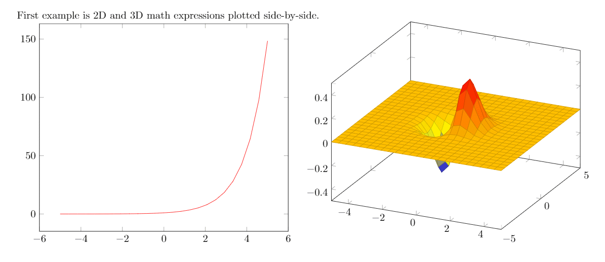
                        \documentclass            {article}            \usepackage            [margin=0.25in]            {geometry}            \usepackage            {pgfplots}            \pgfplotsset            {width=10cm,compat=1.nine}            % We will externalize the figures            \usepgfplotslibrary            {external}            \tikzexternalize            \begin            {document}            Showtime example is 2D and 3D math expressions plotted side-past-side.            %Here begins the 2D plot            \begin            {tikzpicture}            \begin            {axis}            \addplot            [color=red]            {exp(x)};            \end            {axis}            \end            {tikzpicture}            %Hither ends the 2D plot            \hskip            5pt            %Here begins the 3D plot            \begin            {tikzpicture}            \brainstorm            {axis}            \addplot3[     surf, ]            {exp(-x^ii-y^two)*x};            \end            {axis}            \terminate            {tikzpicture}            %Here ends the 3D plot            \end            {document}          

 Open this pgfplots example in Overleaf.

The following image shows the result produced by the code above:

Explanation of the code

Because pgfplots is based on tikz the plot must be inside a tikzpicture environment. Then the environment annunciation \begin{centrality}, \finish{axis} will set the right scaling for the plot—check the Reference guide for other centrality environments.

To add together an actual plot, the command \addplot[color=red]{log(x)}; is used. Within the foursquare brackets, [...], some options can be passed in; here, we set the color of the plot to red. The square brackets are mandatory, if no options are passed leave a blank space between them. Inside the curly brackets y'all put the role to plot. Is important to remember that this command must stop with a semicolon (;).

To put a 2d plot next to the starting time one declare a new tikzpicture surround. Exercise non insert a new line, but a pocket-sized blank gap, in this case hskip 10pt will insert a 10pt-broad blank space.

The rest of the syntax is the same, except for the \addplot3 [surf,]{exp(-x^2-y^2)*x};. This volition add together a 3dplot, and the option surf inside squared brackets declares that information technology'southward a surface plot. The function to plot must be placed inside curly brackets. Once more, don't forget to put a semicolon (;) at the stop of the control.

Annotation: It'southward recommended as a good practice to indent the code—see the 2nd plot in the example above—and to add together a comma (,) at the end of each option passed to \addplot. This fashion the code is more readable and is easier to add further options if needed.

2D plots

pgfplots' 2D plotting functionalities are vast—and you can personalize your plots to adjust your requirements. Nevertheless, the default options usually give very good results, so all yous demand to do is feed the data and LaTeX will do the rest.

Plotting mathematical expressions

Here is an example:

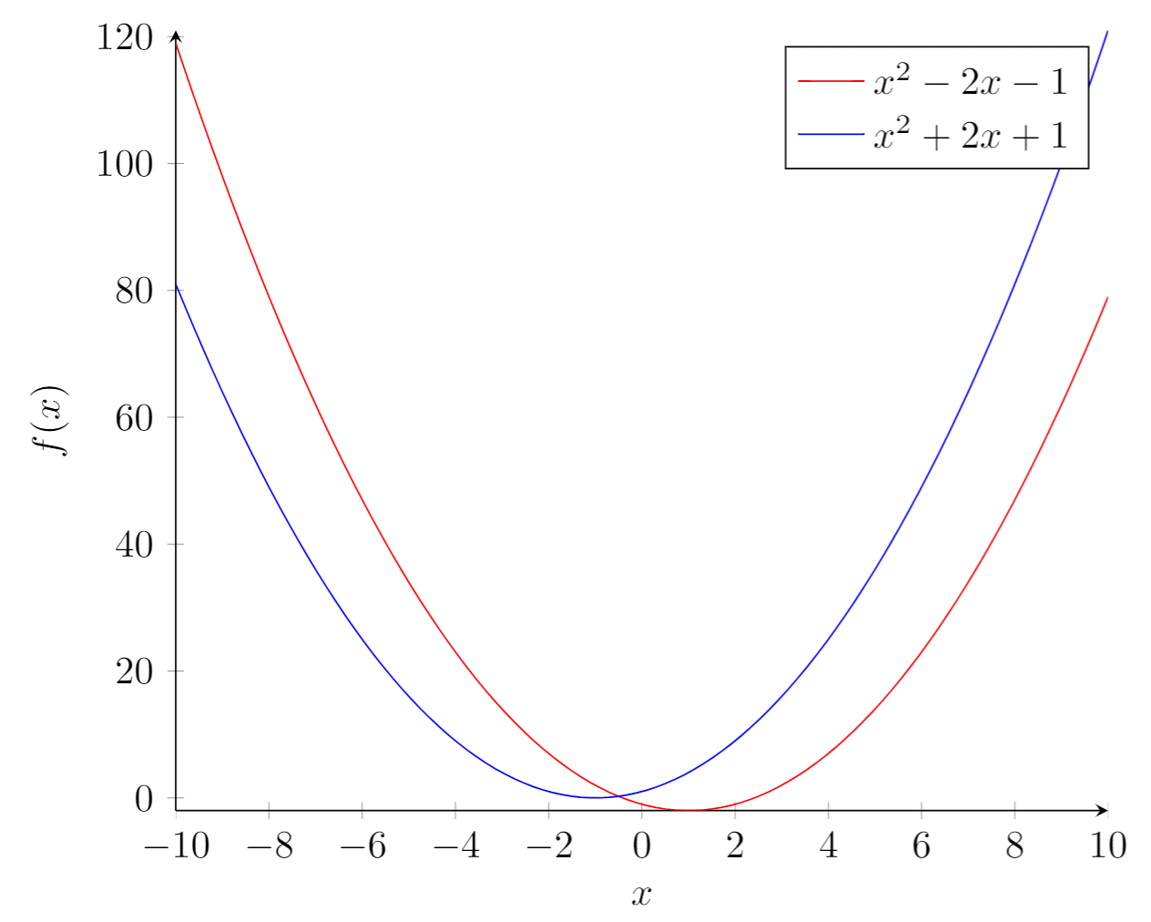
                        \begin            {tikzpicture}            \begin            {axis}[     axis lines = left,     xlabel =            \(            x            \),     ylabel =            {            \(            f            (            10            )            \)            }, ]            %Below the red parabola is divers            \addplot            [     domain=-10:10,      samples=100,      color=red, ]            {10^ii - ii*ten - 1};            \addlegendentry            {            \(            10^            2                                    -                                    2            ten                        -                                    1            \)            }            %Hither the blue parabola is defined            \addplot            [     domain=-10:10,      samples=100,      colour=bluish,     ]            {x^2 + 2*x + 1};            \addlegendentry            {            \(            x^            2                                    +                                    ii            x                        +                                    i            \)            }            \end            {centrality}            \end            {tikzpicture}          

 Open this pgfplots example in Overleaf.

The output from this lawmaking is shown in the image below—the LaTeX document preamble is added automatically when you open up the link:

Explanation of the code

Let'south analyse the new commands line-by-line:

axis lines = left.

This will ready the axis only on the left and bottom sides of the plot, instead of the default box. Farther customisation options at the reference guide.

xlabel = \(x\) and ylabel = {\(f(x)\)}.

Self-explanatory parameter names, these will let yous put a label on the horizontal and vertical axis. Observe the ylabel value in between curly brackets, this brackets tell pgfplots how to group the text. The xlabel could take had brackets also. This is useful for complicated labels that may confuse pgfplots.

\addplot.

This will add a plot to the axis, general usage was described at the introduction. There are 2 new parameters in this case.

domain=-10:10.

This establishes the range of values of \(x\).

samples=100.

Determines the number of points in the interval defined past domain. The greater the value of samples the sharper the graph y'all go, but information technology volition have longer to return.

\addlegendentry{\(x^2 - 2x - i\)}.

This adds the legend to place the function \(x^2 - 2x - one\).

To add another graph to the plot just write a new \addplot entry.

Plotting from data

Scientific research often yields data that has to exist analysed. The next instance shows how to plot data with pgfplots:

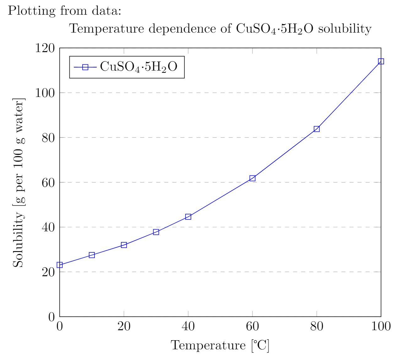
            Plotting from information:            \begin            {tikzpicture}            \begin            {axis}[     championship={Temperature dependence of CuSO\(            _            4            \cdot            \)5H\(            _            2            \)O solubility},     xlabel={Temperature [\textcelsius]},     ylabel={Solubility [g per 100 g h2o]},     xmin=0, xmax=100,     ymin=0, ymax=120,     xtick={0,twenty,xl,60,lxxx,100},     ytick={0,20,twoscore,lx,80,100,120},     legend pos=north west,     ymajorgrids=true,     grid manner=dashed, ]            \addplot[     color=blue,     marking=square,     ]     coordinates            {            (0,23.1)(10,27.5)(20,32)(30,37.8)(40,44.half dozen)(60,61.8)(80,83.8)(100,114)            };            \legend            {CuSO\(            _            4            \cdot            \)5H\(            _            two            \)O}            \end            {axis}            \end            {tikzpicture}          

 Open up this pgfplots example in Overleaf.

The output from this code is shown in the paradigm below—the LaTeX certificate preamble is added automatically when you open the link:

Caption of the lawmaking

There are some new commands and parameters here:

title={Temperature dependence of CuSO\(_4\cdot\)5H\(_2\)O solubility}.

Equally y'all might expect, assigns a title to the figure. The title volition exist displayed above the plot.

xmin=0, xmax=100, ymin=0, ymax=120.

Minimum and maximum bounds of the x and y axes.

xtick={0,20,forty,60,fourscore,100}, ytick={0,20,40,60,eighty,100,120}.

Points where the marks are placed. If empty the ticks are ready automatically.

legend pos=north west.

Position of the legend box. Check the reference guide for more options.

ymajorgrids=truthful.

This Enables/disables grid lines at the tick positions on the y axis. Use xmajorgrids to enable filigree lines on the x centrality.

grid style=dashed.

Self-explanatory. To display dashed grid lines.

mark=foursquare.

This draws a squared marking at each point in the coordinates assortment. Each mark will be connected with the next one past a straight line.

coordinates {(0,23.1)(x,27.v)(20,32)...}

Coordinates of the points to exist plotted. This is the data you want analyse graphically.

If the information is in a file, which is the case most of the time; instead of the commands \addplot and coordinates you should utilise \addplot table {file_with_the_data.dat}, the rest of the options are valid in this environs.

Scatter plots

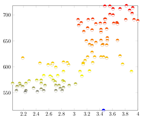
Besprinkle plots are used to represent information by using some kind of marks and are normally used when computing statistical regression. In this example we'll create a scatter plot using data independent in a file called scattered_example.dat, in which the information looks like this:

GPA  ma  ve  co   un 3.45 643 589 3.76 3.52 2.78 558 512 2.87 2.91 2.52 583 503 two.54 2.4 iii.67 685 602 3.83 3.47 3.24 592 538 3.29 3.47 2.1 562 486 2.64 2.37 ...        

Our scatter plot uses the get-go two columns of the data:

                        \begin            {tikzpicture}            \begin            {axis}[     enlargelimits=imitation, ]            \addplot+[     only marks,     scatter,     marking=halfcircle*,     marking size=2.9pt] tabular array[meta=ma]            {scattered_instance.dat};            \terminate            {axis}            \end            {tikzpicture}          

 Open up a scatter plot project case in Overleaf (contains the data file scattered_example.dat).

Explanation of the code

The parameters passed to the axis and addplot environments tin as well be used in a data plot, except for scatter. Beneath the description of the code:

enlarge limits=false

This will shrink the axes so the signal with maximum and minimum values lay on the edge of the plot.

but marks

Really explicit, will put a mark on each point.

scatter

When scatter is used the points are coloured depending on a value, the color is given by the meta parameter explained below.

mark=halfcircle*

The kind of marker to use on each signal, bank check the reference guide for a list of possible values.

marker size=2.9pt

The size of each mark, unlike units can exist used.

table[meta=ma]{scattered_example.dat};

Hither the tabular array command tells latex that the data to be plotted is in a file. The meta=ma parameter is passed to choose the cavalcade that determines the colour of each point. Inside curly brackets is the proper name of the data file.

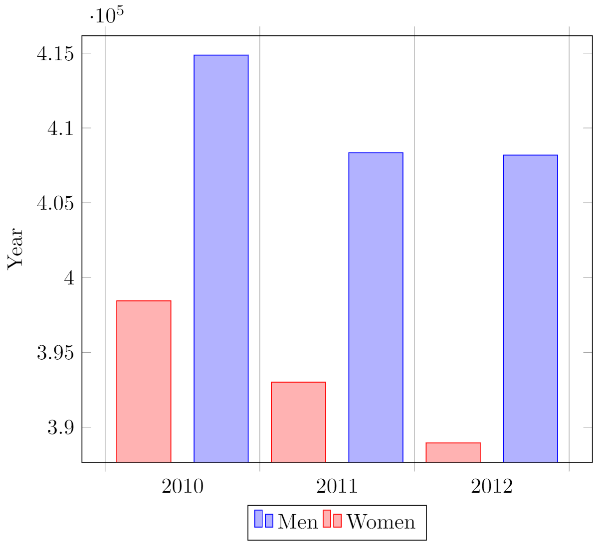
Bar graphs

Bar graphs (as well known equally bar charts and bar plots) are used to display gathered data, mainly statistical data virtually a population of some sort. Bar plots in pgfplots are highly configurable, but here we are going to testify a plain example:

                        \begin            {tikzpicture}            \begin            {axis}[ 	x tick label style={            /pgf/number format/1000 sep=}, 	ylabel=Year, 	enlargelimits=0.05, 	legend style={at={(0.five,-0.one)}, 	anchor=n,legend columns=-1}, 	ybar interval=0.seven, ]            \addplot            coordinates            {(2012,408184) (2011,408348) 		 (2010,414870) (2009,412156)};            \addplot            coordinates            {(2012,388950) (2011,393007)  		(2010,398449) (2009,395972)};            \legend            {Men,Women}            \end            {axis}            \stop            {tikzpicture}          

 Open this pgfplots bar code case in Overleaf.

The output from this code is shown in the image beneath—the LaTeX document preamble is added automatically when you open the link:

Explanation of the code

The figure starts with the (previously explained) declaration of the tikzpicture and axis environments, only the axis announcement has a number of new parameters:

x tick label style={/pgf/number format/thou sep=}

This slice of code defines a complete manner for the plot. With this style yous may include several \addplot commands within this axis environment, they volition fit and look nice together with no farther tweaks (the ybar parameter described below is mandatory for this to work).

enlargelimits=0.05.

Enlarging the limits in a bar plot is necessary because these kind of plots ofttimes crave some extra space in a higher place the bar to expect meliorate and/or add a label. Then number 0.05 is relative to the total height of of the plot.

legend style={at={(0.5,-0.2)}, anchor=north,fable columns=-1}

Again, this will work just fine well-nigh of the time. If anything, change the value of -0.2 to locate the legend closer/further from the ten-centrality.

ybar interval=0.seven,

Thickness of each bar. 1 pregnant the bars volition be i next to the other with no gaps and 0 meaning there will exist no bars, simply only vertical lines.

The coordinates in this kind of plot determine the base point of the bar and its height.

The labels on the y-axis volition prove upward to 4 digits. If the numbers you lot are working with are greater than 9999 pgfplots will use the same annotation as in the instance.

3D Plots

pgfplots has the 3D Plotting capabilities that y'all may await in a plotting software.

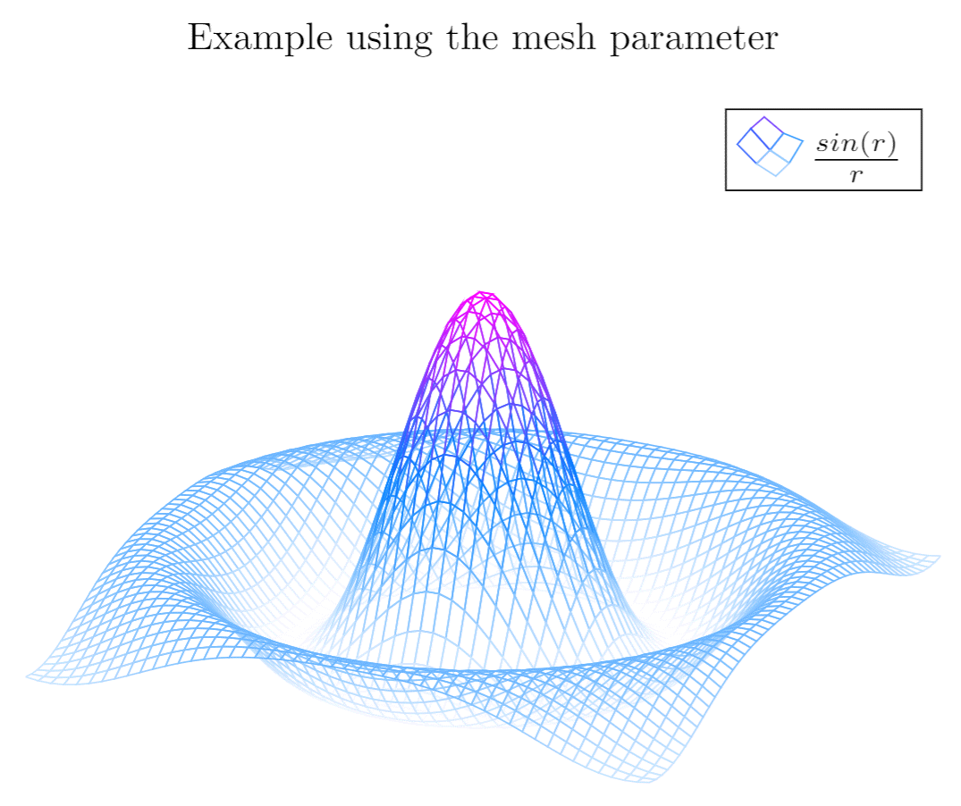
Plotting mathematical expressions

In that location's a uncomplicated example about this at the introduction, let'southward work on something slightly more than circuitous:

                        \begin            {tikzpicture}            \begin            {axis}[     title=Instance using the mesh parameter,     hide axis,     colormap/absurd, ]            \addplot3[     mesh,     samples=fifty,     domain=-viii:8, ]            {sin(deg(sqrt(10^ii+y^two)))/sqrt(10^two+y^ii)};            \addlegendentry            {            \(            \frac            {sin            (            r            )            }{r}            \)            }            \end            {centrality}            \stop            {tikzpicture}          

 Open up this pgfplots 3D example in Overleaf.

The output from this code is shown in the paradigm below—the LaTeX document preamble is added automatically when yous open the link:

Explanation of the code

Near of the commands hither have already been explained, but there are 3 new things:

hide axis

This selection in the axis environment is self descriptive, the axis won't be shown.

colormap/cool

Is the color scheme to be used in the plot. Check the reference guide for more color schemes.

mesh

This option is self-descriptive too, check too the surf parameter in the introductory example.

Note: When working with trigonometric functions pgfplots uses degrees as default units, if the angle is in radians (as in this case) you have to utilise the deg part to catechumen to degrees.

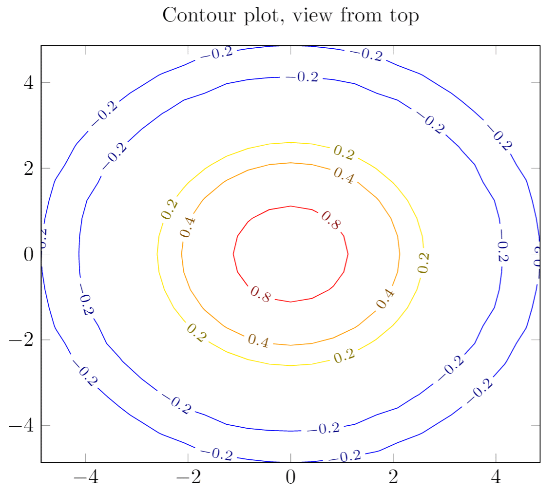
Contour plots

In pgfplots it is possible to plot profile plots, but the data has to be pre-calculated by an external program. Let'due south come across an example:

                        \begin            {tikzpicture}            \brainstorm            {centrality}            [     championship={Contour plot, view from tiptop},     view={0}{90}            ]            \addplotiii[     contour gnuplot={levels={0.8, 0.4, 0.two, -0.ii}}            ]            {sin(deg(sqrt(x^2+y^2)))/sqrt(ten^ii+y^2)};            \end            {axis}            \end            {tikzpicture}          

 Open up this pgfplots contour plot example in Overleaf.

The output from this code is shown in the epitome beneath—the LaTeX document preamble is added automatically when you open up the link:

Explanation of the code

This is a plot of some contour lines for the aforementioned equation used in the previous section. The value of the title parameter is inside curly brackets because it contains a comma, so nosotros employ the grouping brackets to avert any defoliation with the other parameters passed to the \begin{centrality} announcement. At that place are two new commands:

view={0}{ninety}

This changes the view of the plot. The parameter is passed to the axis surroundings, which means this can be used in whatsoever other type of 3D plot. The get-go value is a rotation, in degrees, around the z-axis; the second value is to rotate the view around the 10-centrality. In this case when we combine a 0° rotation around the z-axis and a ninety° rotation around the x-axis we end upward with a view of the plot from meridian.

contour gnuplot={levels={0.viii, 0.iv, 0.2, -0.2}}

This line of lawmaking does two things: First, it tells LaTeX to use the external software gnuplot to compute the contour lines; this works fine in Overleaf but if you want to use this command in your local LaTeX installation you accept to install gnuplot first (matlab will too work, in such instance write matlab instead of gnuplot in the command). 2d, the sub parameter levels is a list of values of acme levels where the contour lines are to be computed.

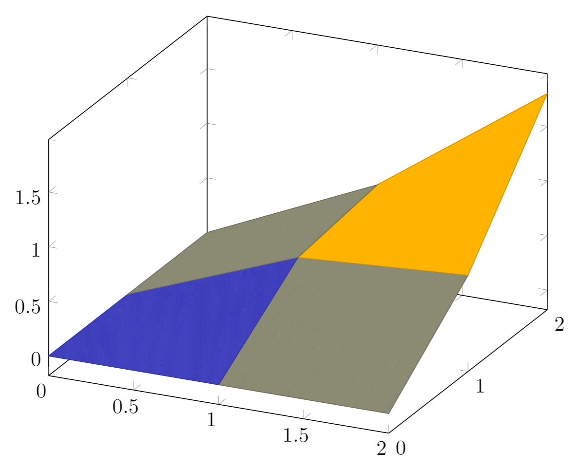
Plotting a surface from data

To plot a set of data into a 3D surface all we need is the coordinates of each indicate. These coordinates could exist an unordered set or, in this case, a matrix:

                        \begin            {tikzpicture}            \begin            {centrality}            \addplot3[     surf, ]  coordinates            {            (0,0,0) (0,ane,0) (0,ii,0)  (1,0,0) (1,one,0.6) (1,two,0.seven)  (two,0,0) (two,1,0.7) (2,2,1.8)            };            \end            {axis}            \stop            {tikzpicture}          

 Open this pgfplots 3D surface example in Overleaf.

The output from this lawmaking is shown in the image beneath—the LaTeX document preamble is added automatically when you open the link:

Caption of the data

The points passed to the coordinates parameter are treated every bit contained in a 3 × 3 matrix, using a blank line every bit the separator for each matrix row.

All the options for 3D plots in this article apply to information surfaces.

Parametric plot

The syntax for parametric plots is slightly unlike. Let'southward see an example:

                        \begin            {tikzpicture}            \begin            {axis}            [     view={lx}{30},     ]            \addplotiii[     domain=0:5*pi,     samples = lx,     samples y=0, ] ({sin(deg(x))},            {cos(deg(ten))},            {x});            \end            {axis}            \finish            {tikzpicture}          

 Open this pgfplots parametric plot example in Overleaf.

The output from this lawmaking is shown in the image below—the LaTeX document preamble is added automatically when yous open the link:

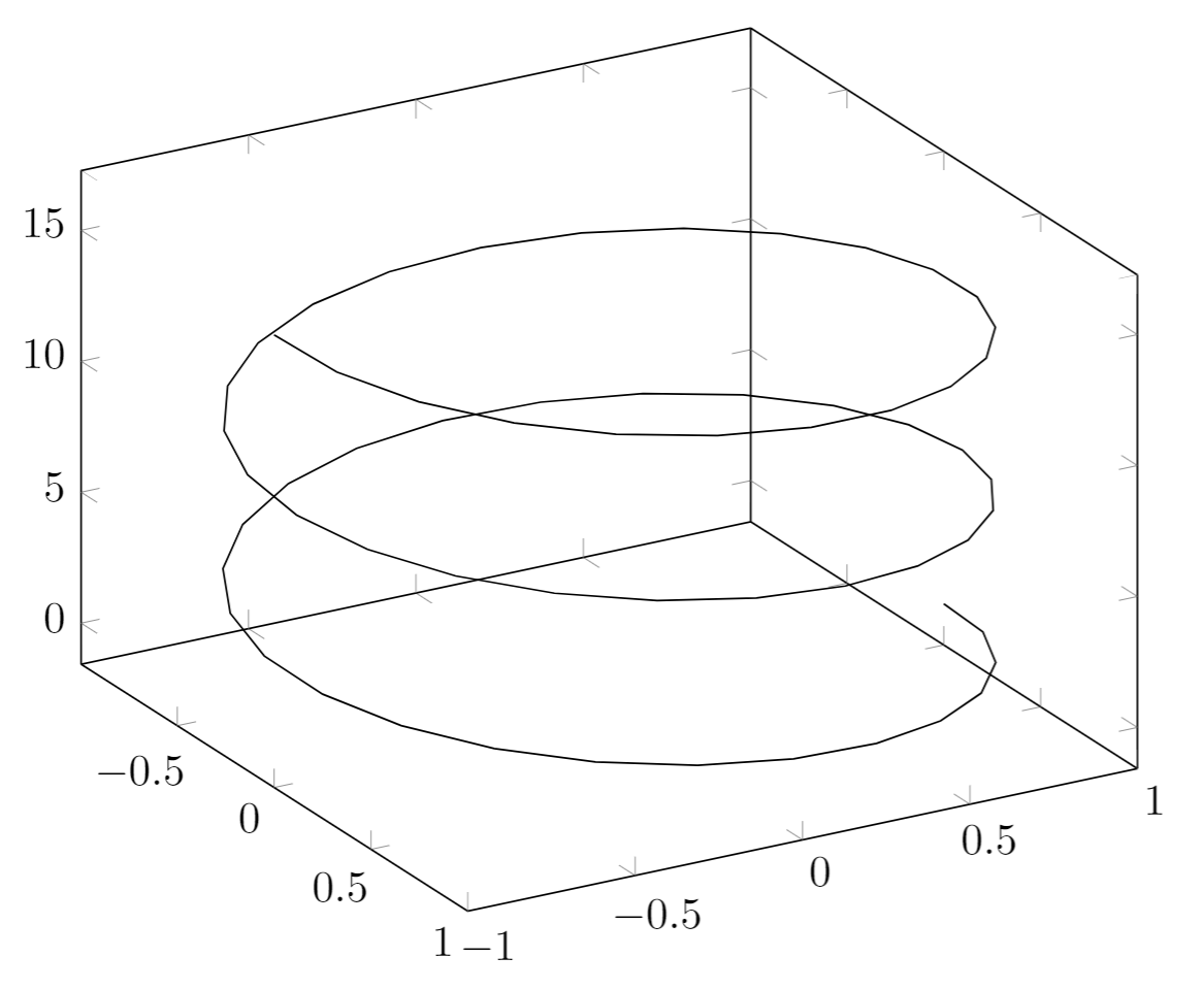
Explanation of the code

In that location are only 2 new things in this example: beginning, the samples y=0 to prevent pgfplots from joining the extreme points of the screw and; second, the way the function to plot is passed to the addplot3 environment. Each parameter function is grouped inside curly brackets and the three parameters are delimited with a parenthesis.

Reference guide

Command/Pick/Surroundings	Description	Possible Values
axis	Normal plots with linear scaling
semilogxaxis	logarithmic scaling of x and normal scaling for y
semilogyaxis	logarithmic scaling for y and normal scaling for x
loglogaxis	logarithmic scaling for the x and y axes
centrality lines	changes the fashion the axes are drawn. default is 'box	box, left, middle, middle, right, none
legend pos	position of the fable box	s due west, south east, north due west, due north east, outer north east
marking	blazon of marks used in data plotting. When a single-grapheme is used, the character advent is very similar to the actual marking.	*, x , +, |, o, asterisk, star, 10-pointed star, oplus, oplus*, otimes, otimes*, square, square*, triangle, triangle*, diamond, halfdiamond*, halfsquare*, right*, left*, Mercedes star, Mercedes star flipped, halfcircle, halfcircle*, pentagon, pentagon*, cubes. (cubes simply work on 3d plots).
colormap	colour scheme to exist used in a plot, can be personalized but at that place are some predefined colormaps	hot, hot2, jet, blackwhite, bluered, absurd, greenyellow, redyellow, violet.

Further reading

For more than information see:

• Using colours in LaTeX
• TikZ package
• Externalising pgfplots and tikzpictures
• Inserting Images
• Lists of tables and figures
• Positioning images and tables
• Cartoon diagrams directly in LaTeX
• The pgfplots parcel documentation.
• The TikZ and PGF Packages: Transmission for version iii.0.0
• TikZ and PGF examples at TeXample.net

Source: https://www.overleaf.com/learn/latex/Pgfplots_package

Posted by: steadmanpilly1987.blogspot.com

Share this post